Forecasting PM2.5 with forecast and prophet

Data Collection

The pollution data I’ll be using for this examples comes from epa.gov and the weather data comes from ncdc.noaa.gov. You can access my R data object on my github page. Salt Lake City for many years has experienced population growth which has exasterbated the inversion problem. Inversion creates a “cap” over Utah valleys trapping pollutants on the valley floors which creates many public health issues because of the thick smog.

Below is an map indicating 4 sites where data is being collected on pollution levels. I will be focusing particulary on PM2.5 measures across the Salt Lake Valley. I’ve also downloaded weather data from both the valley floor at SLC International Airport and in a meadow near Grand View peak in the Wasatch mountains. These two sites’ temperatures can be used to compute whether the temperatures are inverted.

OLS Regression

First, let’s take a look at how well our weather regressors are at predicting PM2.5 levels without considering autocorrelation or seasonality. Below, we will fit our model and look at our residuals to make sure our assumptions of normality and independence are met:

fit1 <- lm(sqrt(pm2.5)~inversion+wind+precip+fireworks,data=dat)
summary(fit1)

## 
## Call:
## lm(formula = sqrt(pm2.5) ~ inversion + wind + precip + fireworks, 
##     data = dat)
## 
## Residuals:
##     Min      1Q  Median      3Q     Max 
## -2.1571 -0.5555 -0.1835  0.3608  4.4629 
## 
## Coefficients:
##              Estimate Std. Error t value Pr(>|t|)    
## (Intercept)  3.322431   0.066358  50.068  < 2e-16 ***
## inversion    2.527237   0.130122  19.422  < 2e-16 ***
## wind        -0.040543   0.003255 -12.454  < 2e-16 ***
## precip      -0.515741   0.175563  -2.938  0.00336 ** 
## fireworks    0.545624   0.116089   4.700 2.85e-06 ***
## ---
## Signif. codes:  0 '***' 0.001 '**' 0.01 '*' 0.05 '.' 0.1 ' ' 1
## 
## Residual standard error: 0.8791 on 1456 degrees of freedom
## Multiple R-squared:  0.3165, Adjusted R-squared:  0.3146 
## F-statistic: 168.5 on 4 and 1456 DF,  p-value: < 2.2e-16

dat$resid[!is.na(dat$pm2.5)] <- resid(fit1)

# Plot the residuals
ggplot(dat,aes(date,resid)) + 
  geom_point() + geom_smooth() +
  ggtitle("Linear Regression Residuals",
          subtitle = paste0("RMSE: ",round(sqrt(mean(dat$resid^2,na.rm=TRUE)),2)))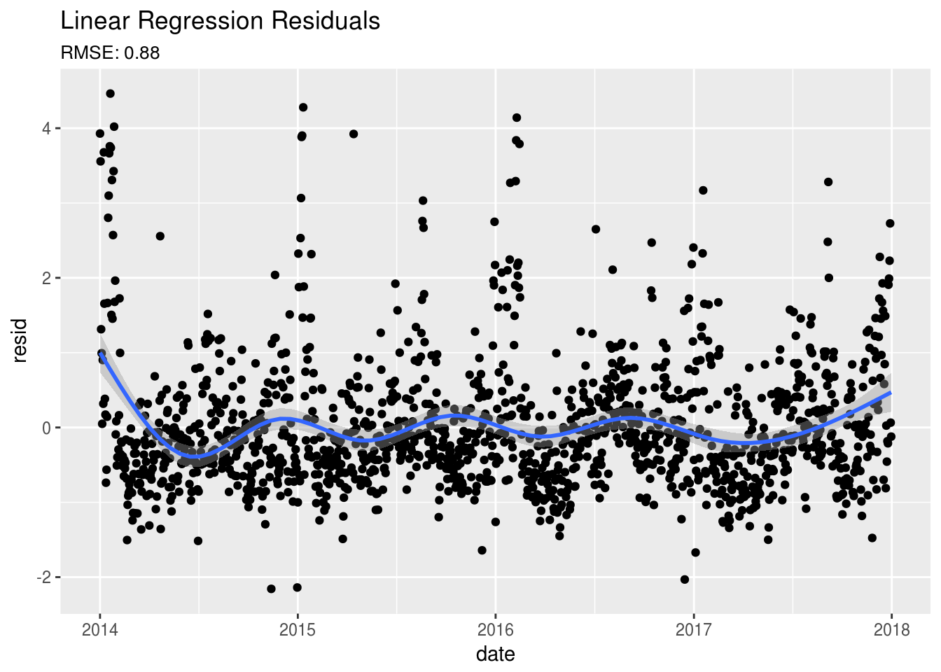

Okay, so when we review the model we see that the variables are somewhat useful in predicting PM2.5 levels, however our r-squared values are not that impressive. Also, looking at our residuals, we can see that there is still something going on that we haven’t accounted for. There appears to be a yearly pattern in the residuals. As for investigating dependece between the PM2.5 data points, let’s use the autocorrelation function, Acf() available in the forecast package:

Acf(dat$resid, main="ACF of OLS Residuals")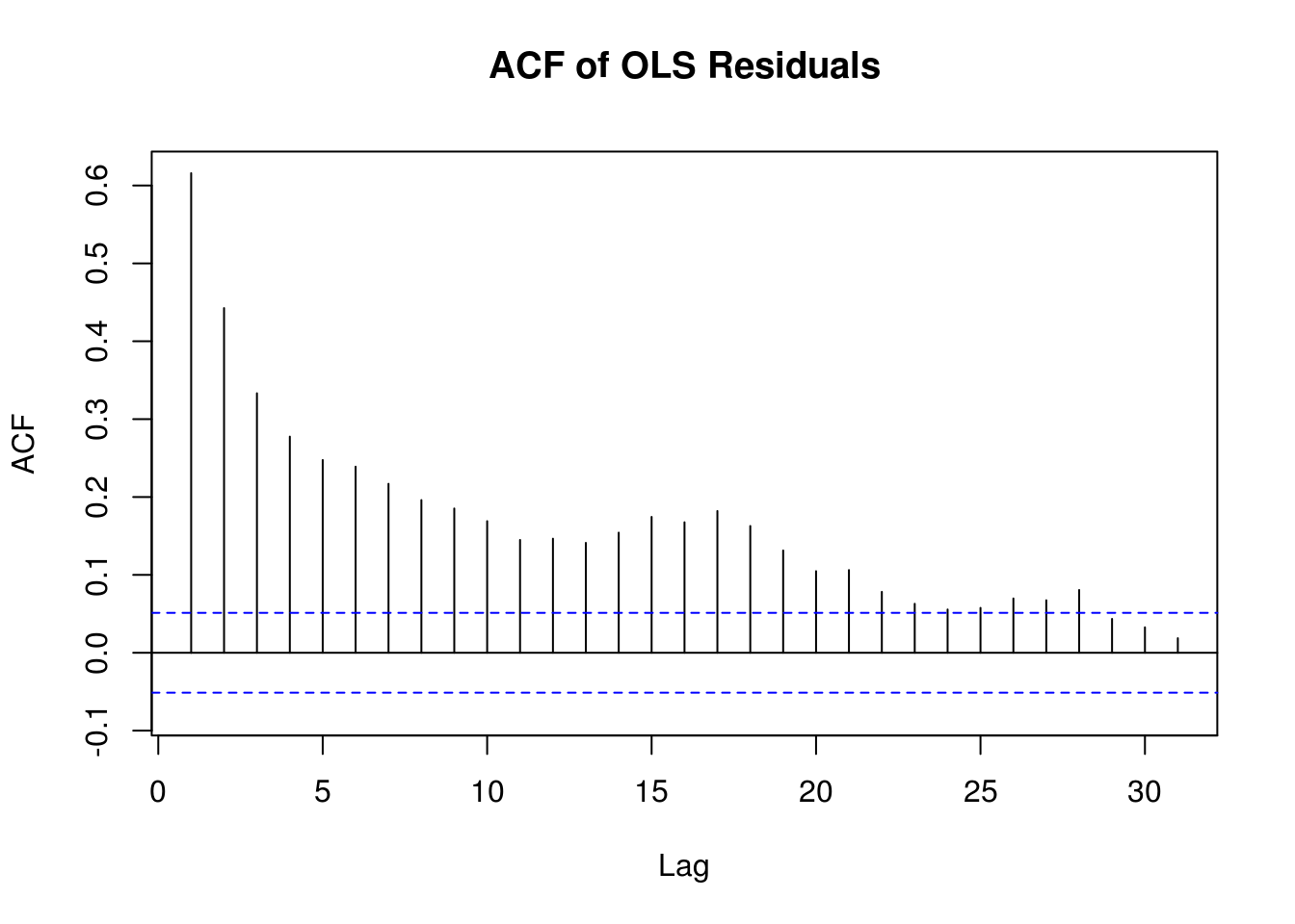

Here we can see that the data is correlated up through 20 or more days in the past. This definitely violates our assumption of independence.

Random Forest Regression

Random Forest models don’t have as many assumptions as OLS Regression, so let’s try this model to see if we can do any better. Initially I’ll be using the training Root Mean Squared Errors (RMSE) to compare models. However, later I will use time series cross-validation RMSE to compare each of the methods ability to predict future PM2.5 levels.

fit2 <- randomForest(sqrt(pm2.5)~inversion+wind+precip+fireworks,data=dat[!is.na(dat$pm2.5),], ntree=500)
dat$rf.resid[!is.na(dat$pm2.5)] <- fit2$predicted - sqrt(dat$pm2.5[!is.na(dat$pm2.5)])

# Plot the residuals
ggplot(dat,aes(date,rf.resid)) + 
  geom_point() + geom_smooth() +
  ggtitle("Random Forest Residuals",
          subtitle = paste0("RMSE: ",round(sqrt(fit2$mse[500]),2)))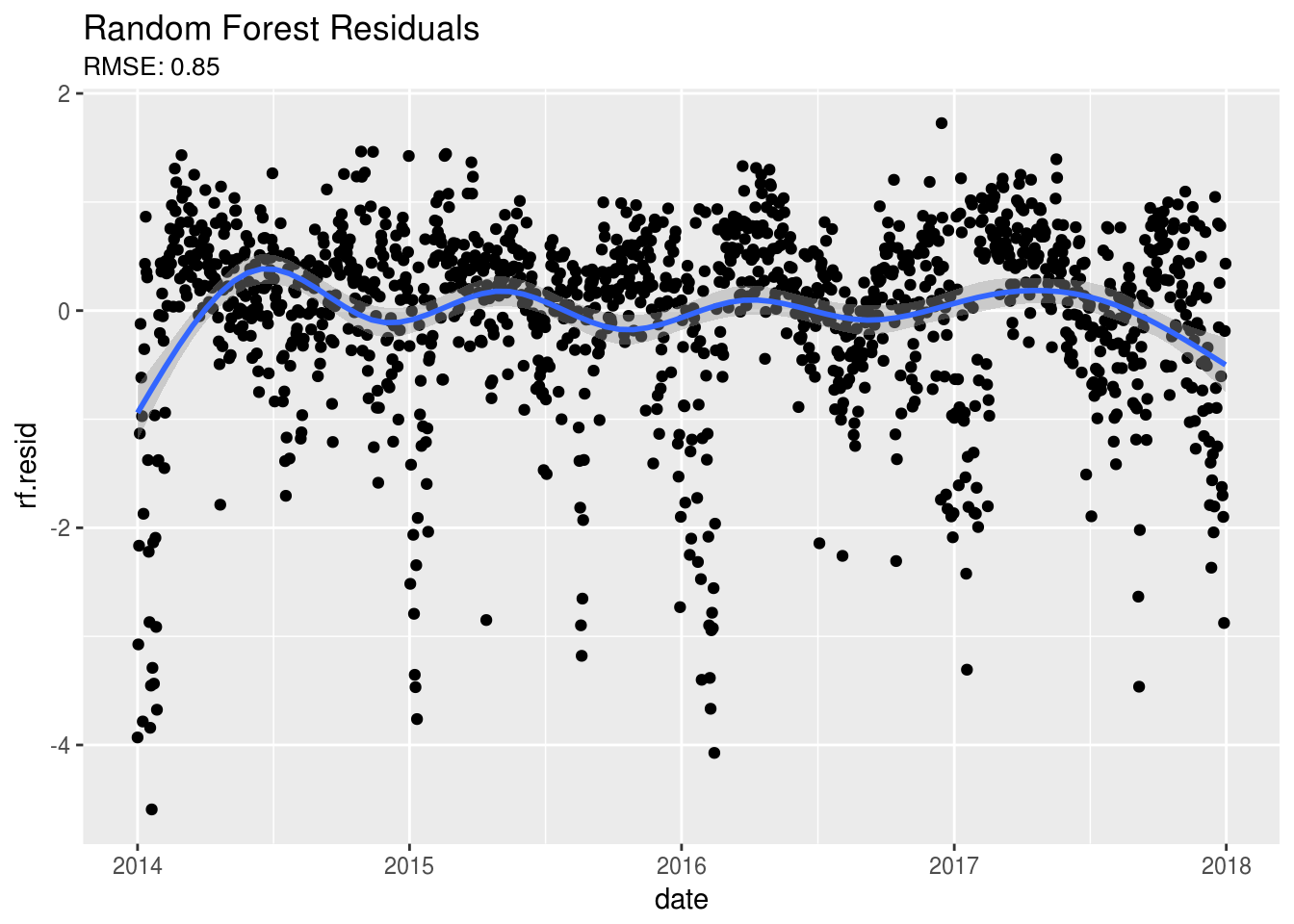

# Better but we still have some odd things going on in our data

Once again, after looking at the residuals it still looks like something is going on here. We notice that there still appears to be a seasonal trend in our residuals. Let’s zoom in on the residual plots over time and take a look:

# Zoom In
p1 <- ggplot(dat,aes(date,rf.resid)) + 
  geom_point() + geom_line() +
  xlim(as.Date(c("2014-01-01","2014-02-28"))) + 
  geom_abline(slope=0, intercept = 0, lty=2, col = "blue", lwd = 1.25)

p2 <- ggplot(dat,aes(date,rf.resid)) + 
  geom_point() + geom_line() +
  xlim(as.Date(c("2017-11-01","2017-12-31"))) + 
  geom_abline(slope=0, intercept = 0, lty=2, col = "blue", lwd = 1.25)


grid.arrange(p1, p2, ncol=2, top="Zoom-in of Random Forest Residuals")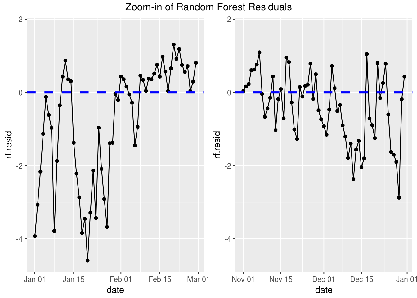

If you look closely it appears that the residuals are all negative for a time then they move to be all positive. From this we see that we still haven’t adjusted our model for the autocorrelation. To do this we’ll need to take a look at some time series models.

Exponential Smoothing

Okay, let’s get started with one of the more simple time series models, Exponential Smoothing. This is done by first converting our target column to a time series object using the ts() function. The ts() function also allows us to include a seasonal component to our data. We’ll start by setting frequency = 7 to include weekly seasonality in our daily PM2.5 measures. In this exercise, I will be fitting 3 different models. The default model argument is set to 'ZZZ' which will choose additive ('A'), multiplicative ('M'), or none ('N') for each of the errors, trend, and seasonality. Our automated model has chosen 'MAN'. Notice that this essentially removed the weekly seasonality which can be seen in the forecast below. I also fit models using all additive and all multiplicative for comparison.

# Convert to time series data
dat.ts <- sqrt(ts(dat[,"pm2.5"], frequency = 7))

# Exponential smoothing model with weekly seasonality
fit3 <- ets(dat.ts) # model = "MAN"
fit4a <- ets(dat.ts, model ="AAA")
fit4b <- ets(dat.ts, model ="MMM")
# Fit models with all additive or all multiplicative features. First byte is for errors, second for trend, and third for seasonality

Notice that similar to linear models, the predict() function is available but can also be used to forecast future values based on previous values by adding an argument for the horizon, h. Below, I’m using the automated ets model to predict 25 days into the future:

# Predict Future Values
plot(predict(fit3,h=25),xlim=c(200,215))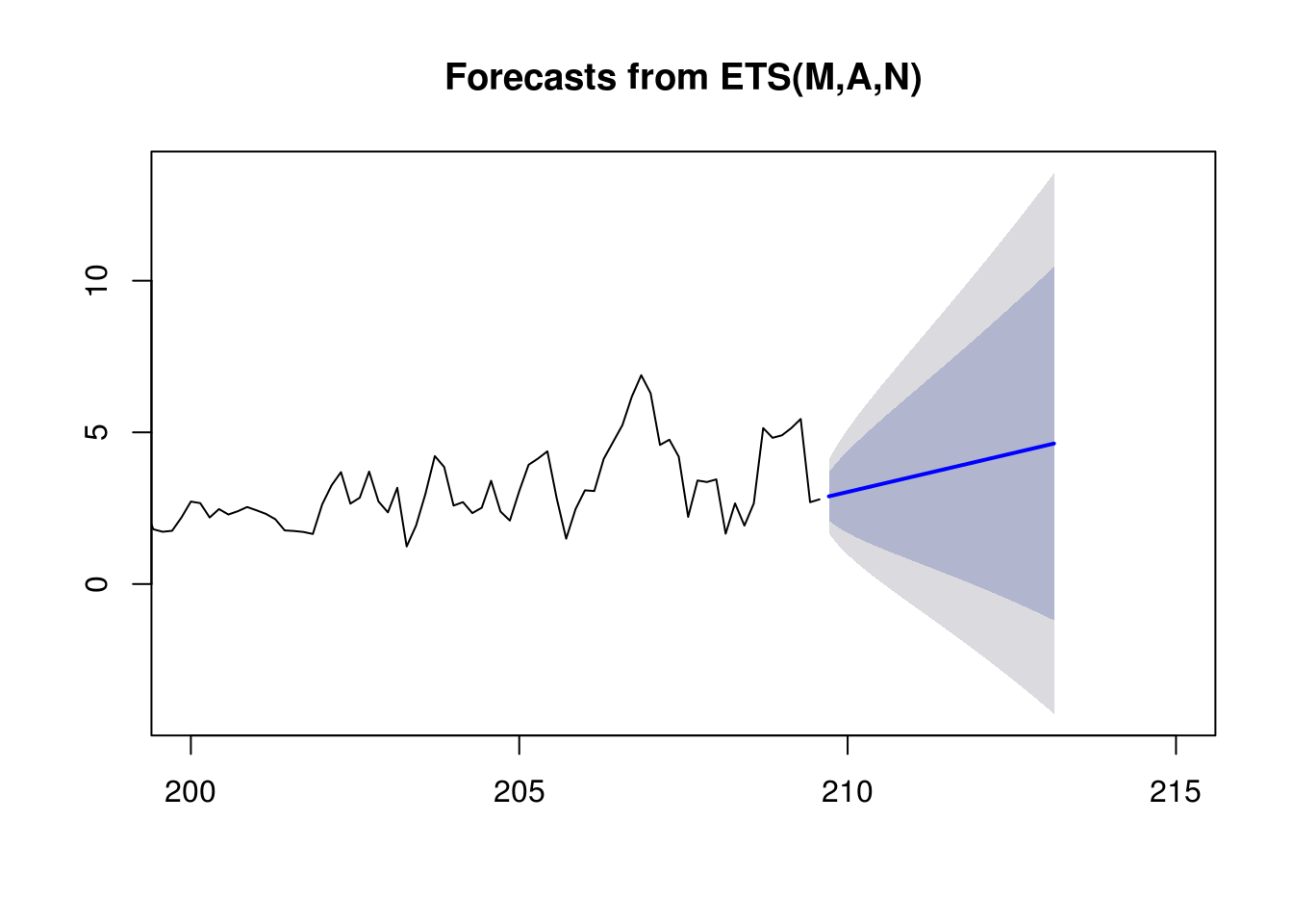

Now going back to our 3 models, we can take a look at the residuals now that we are adjusting for autocorrelation and weekly seasonality:

ets.mod <- rbind(data.frame(day=1:sum(!is.na(dat.ts)), resid=as.numeric(residuals(fit3)), type="Auto"),
                 data.frame(day=1:sum(!is.na(dat.ts)), resid=as.numeric(residuals(fit4a)), type="Additive"),
                 data.frame(day=1:sum(!is.na(dat.ts)), resid=as.numeric(residuals(fit4b)), type="Multiplicative"))

# Compare the residuals of each model
ggplot(ets.mod,aes(day,resid)) + 
  geom_point() + geom_smooth() + 
  facet_grid(type~.,scales="free")+
  ggtitle("ETS Residuals with Weekly Seasonality",
          subtitle = paste0("Auto RMSE: ",round(sqrt(fit3$mse),2),
                            "   Additive RMSE: ",round(sqrt(fit4a$mse),2),
                            "   Multiplicative RMSE: ",round(sqrt(fit4b$mse),2)))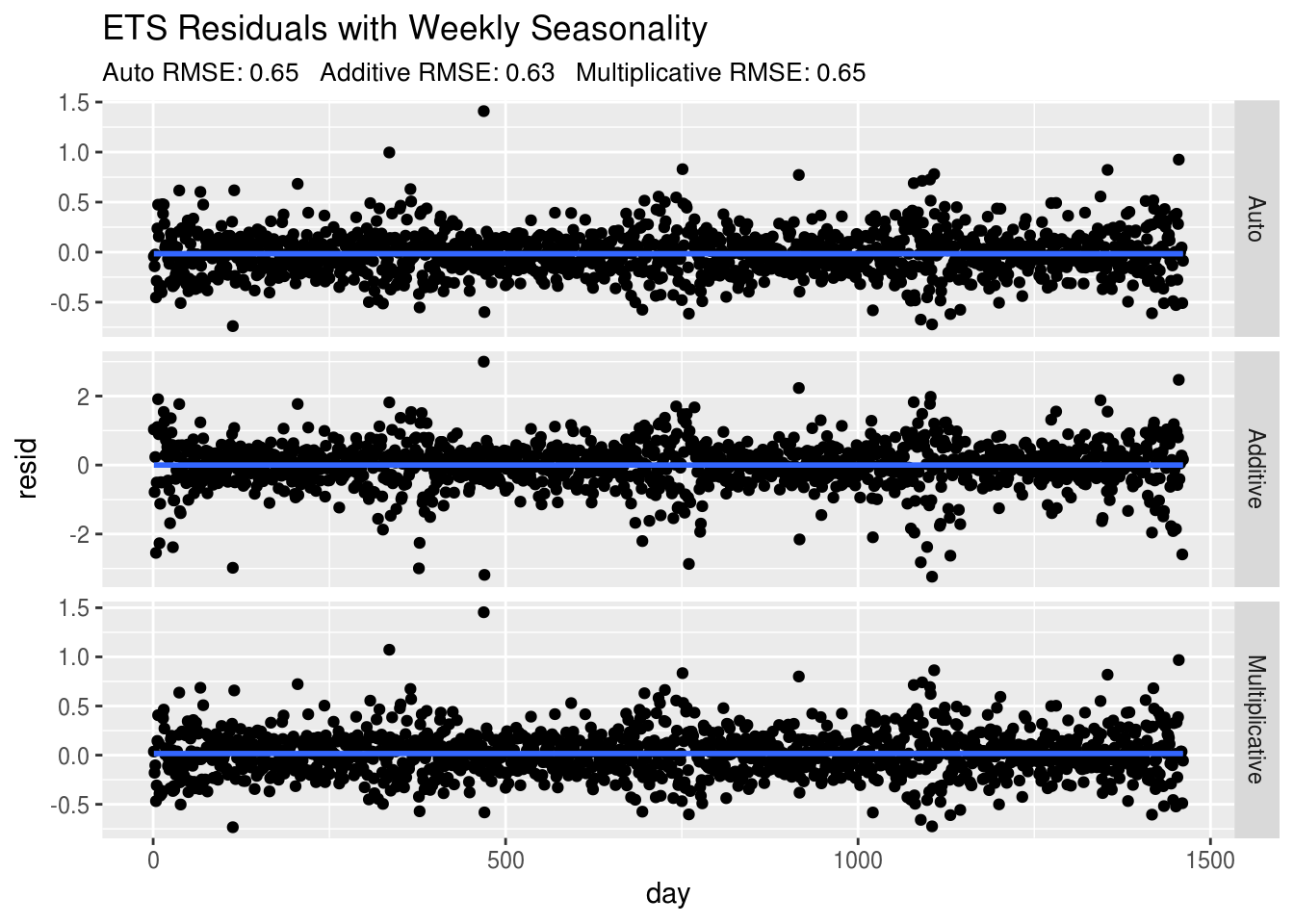

There we go! Our residuals look much better, there still does appear to be some yearly seasonality that we can incorporate using some more sophisticated time series models. Let’s start with Rob Hyndman’s implementation of the TBATS model.

TBATS (Trigonometric regressors, Box-Cox transformations, ARMA errors, Trend, Seasonality)

Using the TBATS model is one way to incorporate multiple seasonality in our model. It’s going to automate the process of choosing a Box-Cox transformation for our target variable, PM2.5. You may have noticed that I’ve been taking the square root of PM2.5 in each of our previous models and this in part was due to the recommended Box-Cox parameter of 0.5 that came out of this model when I was first playing around with the tbats() function. This function will also automatically choose the parameters for the ARMA model and the fourier transforms for the seasonal trends.

# TBATS model with weekly and yearly seasonality
dat.ts2 <- sqrt(msts(dat[!is.na(dat$pm2.5),"pm2.5"], seasonal.periods=c(7,365.25)))
fit5 <- tbats(dat.ts2)
# This method takes the most time when comparing run time.
# Down side on this is that you cannot set specific box-cox, ARMA, and fourier parameters.

This time series model is easy to use and can be extremely useful when modeling mutiple seasonality and autoregressive features. I do wish the tbats() function would allow you to pass specific Box-Cox, ARMA, and fourier parameters for your model. This would make cross-validation of my models more convenient by allowing me to be able to set the specific model for each window.

Once again, you can see that predicting future values is made very easy with the predict() function and h parameter.

# Predict future values
plot(predict(fit5, h=25),xlim=c(4.8,5.2))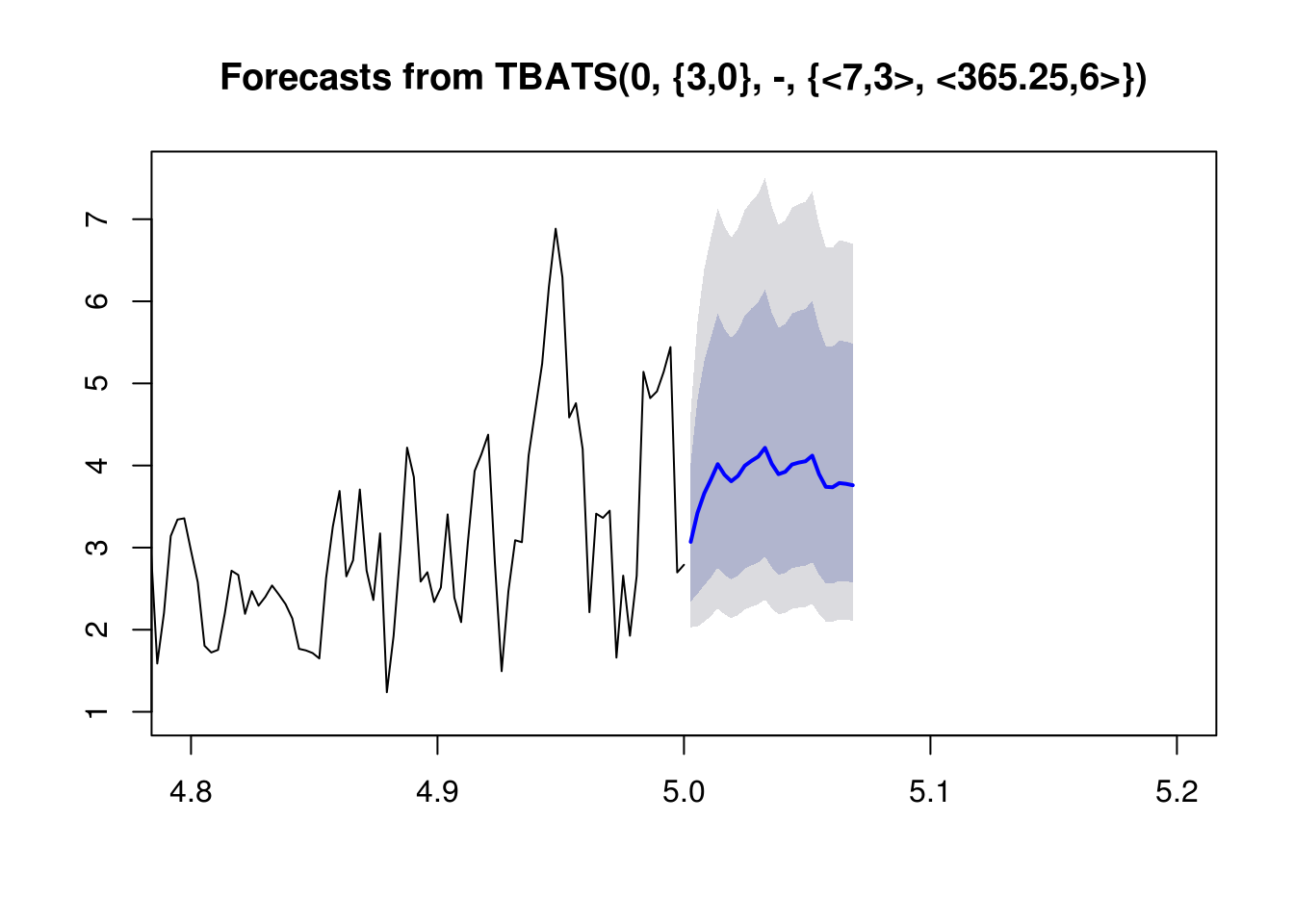

Lastly, let’s look at the residuals and see if adding both yearly and weekly seasonality have improved our predictions:

# Plot the residuals
tbats.mod <- data.frame(day=1:sum(!is.na(dat.ts2)),resid=as.numeric(residuals(fit5)))
ggplot(tbats.mod,aes(day,resid)) + 
  geom_point() + geom_smooth() + 
  ggtitle("TBATS Resids with Dual Seasonality",
          subtitle = paste0("Auto RMSE: ",round(sqrt(mean((residuals(fit5))^2)),2)))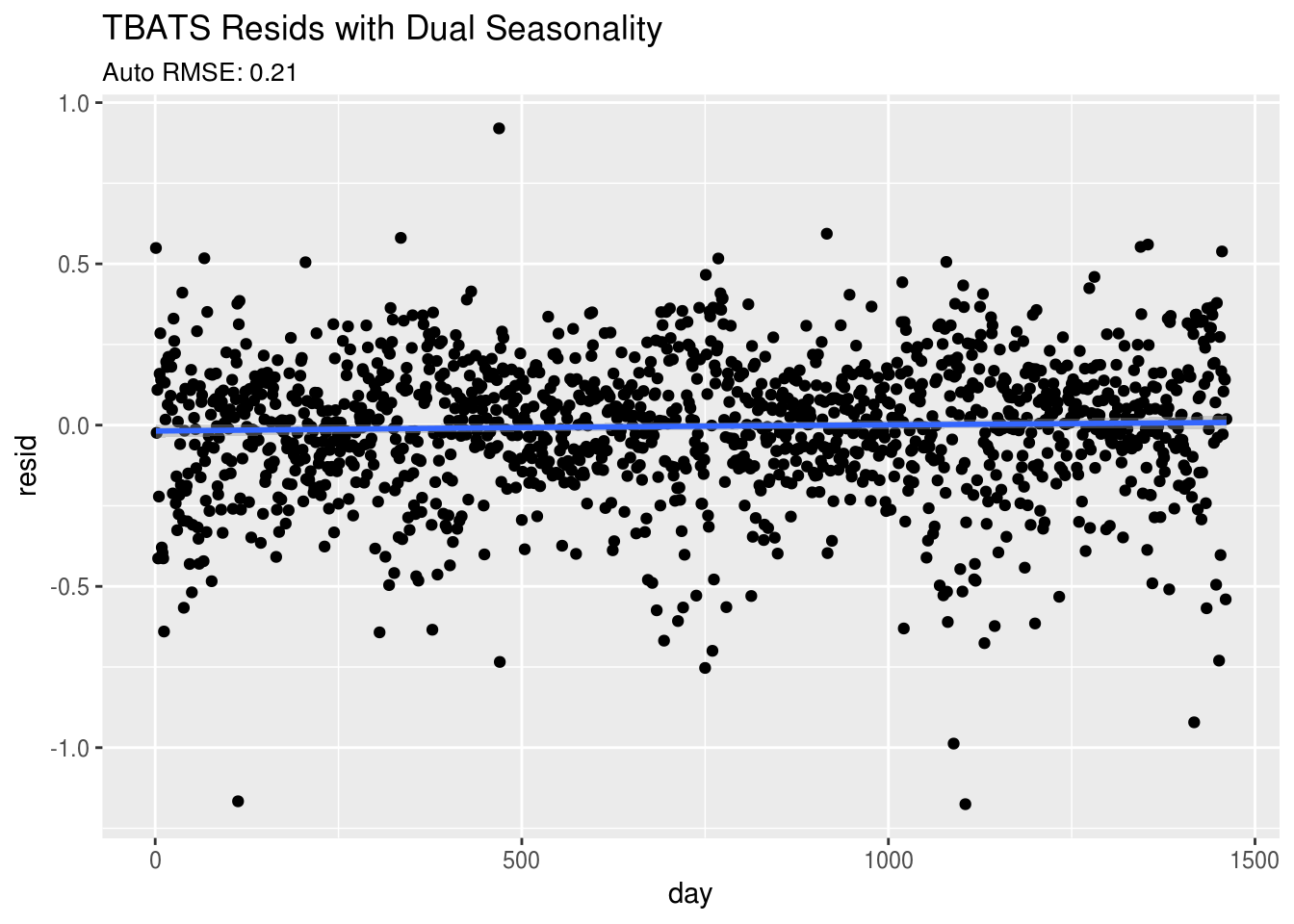

Wow! This looks much better. This random cloud of data around the line y = 0 is typically what we are looking for in a good model fit. Notice also that the training RMSE is much better for this model.

ARIMA with Regressors (AutoRegressive Integraged Moving Average)

The last piece to time series models is being able to add regressors to the multiple seasonality and autocorrelation adjustments. The auto.arima() function can have all of these included in the model by using the fourier() transform function and the xreg argument.

In this portion of the exercise, because my regressors are also time series I need to make sure that I also forcast each of those regressors before using them to forecast the PM2.5 level.

# ARIMA with weekly and yearly seasonality with regressors
regs <- dat[!is.na(dat$pm2.5),c("precip","wind","inversion","fireworks")]

# Forecast weather regressors
weather.ts <- msts(dat[,c("precip","wind","inversion_diff")],seasonal.periods = c(7,365.25))
precip <- auto.arima(weather.ts[,1])
fprecip <- as.numeric(data.frame(forecast(precip,h=25))$Point.Forecast)
wind <- auto.arima(weather.ts[,2])
fwind <- as.numeric(data.frame(forecast(wind,h=25))$Point.Forecast)
inversion <- auto.arima(weather.ts[,3])
finversion <- as.numeric(data.frame(forecast(inversion,h=25))$Point.Forecast)

fregs <- data.frame(precip=fprecip,wind=fwind,inversion=as.numeric(finversion<0),fireworks=0)

# Seasonality
z <- fourier(dat.ts2, K=c(2,5))
zf <- fourier(dat.ts2, K=c(2,5), h=25)

# Fit the model
fit <- auto.arima(dat.ts2, xreg=cbind(z,regs), seasonal=FALSE)

# Predict Future Values
# This time we need future values of the regressors as well.
fc <- forecast(fit, xreg=cbind(zf,fregs), h=25)
plot(fc,xlim=c(4.8,5.2))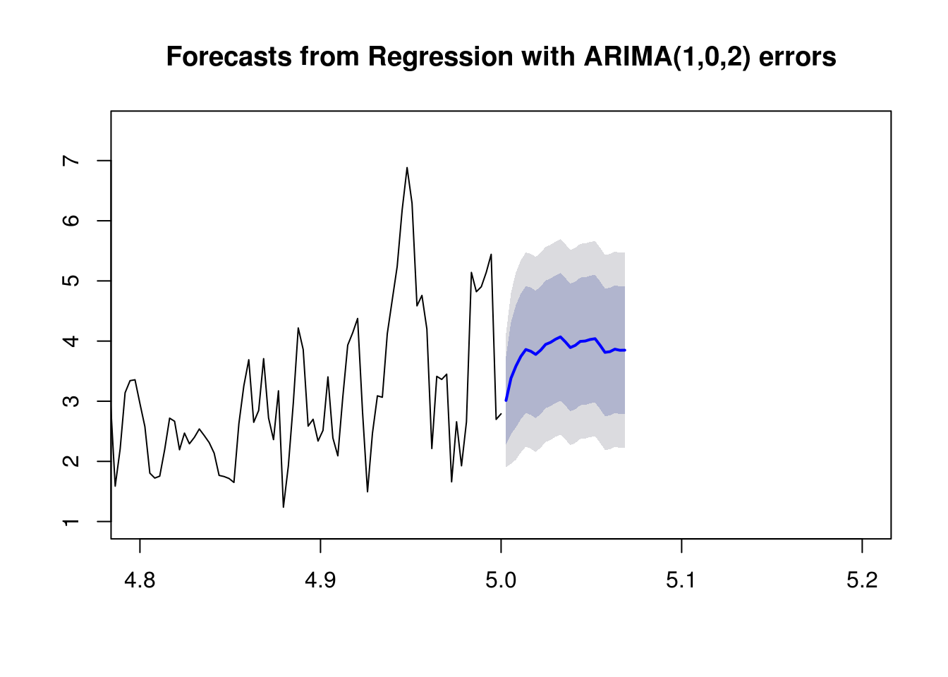

Again, the residuals do look much better than our residuals from the OLS and Random Forest Regression models.

# Plot the residuals
arima.mod <- data.frame(day=1:sum(!is.na(dat.ts)),resid=as.numeric(residuals(fit)))

ggplot(arima.mod,aes(day,resid)) + 
  geom_point() + geom_smooth() + 
  ggtitle("Arima Resids with Seasonality and Regressors",
          subtitle = paste0("RMSE: ",round(sqrt(mean((residuals(fit))^2)),2)))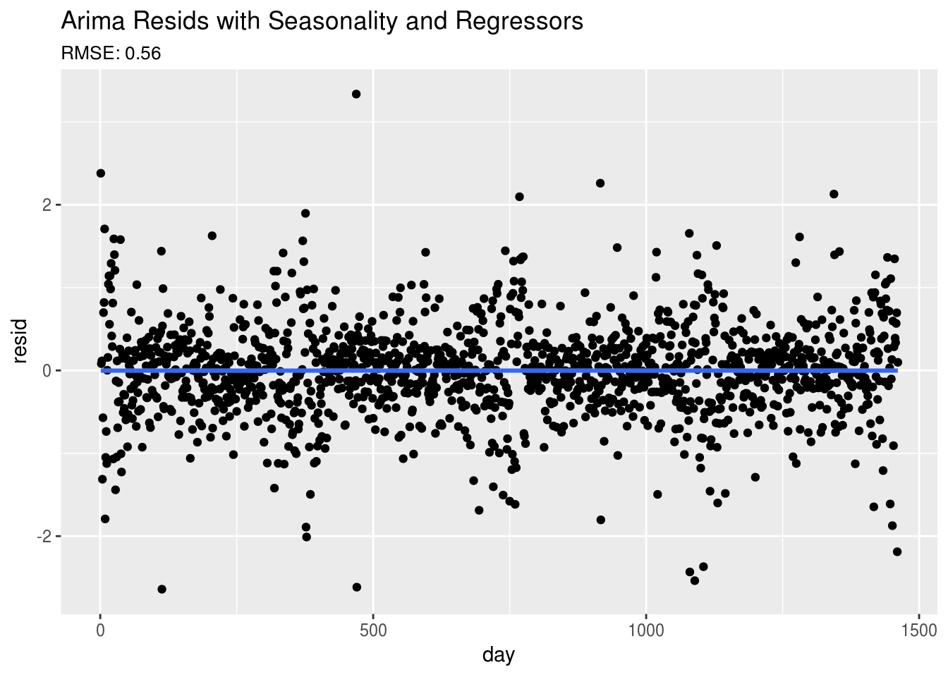

prophet

And finally, let’s take a look at fitting a basic model using the prophet package. The prophet package is using STAN to to fit an additive model by including seasonality, autocorrelation, extra regressors, etc. One of the nice features of the prophet() function is that it will also automatically choose change points in your time series. The default number of change points is set to 25. This allows the time series models to be a little bit more robust in comparison to other models. Once again, I’m also using the prophet() forecast function to forecast my regressors that I’m passing into the final prophet model to predict PM2.5.

pdat <- data.frame(ds=dat$date,
                   y=sqrt(dat$pm2.5),
                   precip=dat$precip,
                   wind=dat$wind,
                   inversion_diff=dat$inversion_diff,
                   inversion=dat$inversion_,
                   fireworks=dat$fireworks)

# Forecast weather regressors
pfdat <- data.frame(ds=max(dat$date) + 1:25)
pprecip <- pdat %>% 
  select(ds,y=precip) %>% 
  prophet() %>%
  predict(pfdat)

## Initial log joint probability = -5.77805
## Optimization terminated normally: 
##   Convergence detected: relative gradient magnitude is below tolerance

pwind <- pdat %>% 
  select(ds,y=wind) %>% 
  prophet() %>%
  predict(pfdat)

## Initial log joint probability = -46.5575
## Optimization terminated normally: 
##   Convergence detected: relative gradient magnitude is below tolerance

pinversion <- pdat %>% 
  select(ds,y=inversion_diff) %>% 
  prophet() %>%
  predict(pfdat)

## Initial log joint probability = -55.0515
## Optimization terminated normally: 
##   Convergence detected: relative gradient magnitude is below tolerance

fdat <-  data.frame(ds=pfdat$ds,
                    precip=pprecip$yhat,
                    wind=pwind$yhat,
                    inversion=as.numeric(pinversion$yhat<0),
                    fireworks = 0)

# Fit the model (Seasonality automatically determined)
fit6 <- prophet() %>% 
  add_regressor('precip') %>% 
  add_regressor('wind') %>% 
  add_regressor('inversion') %>% 
  add_regressor('fireworks') %>% 
  fit.prophet(pdat)

## Initial log joint probability = -120.752
## Optimization terminated normally: 
##   Convergence detected: relative gradient magnitude is below tolerance

We also see that the predict funtion can also be used with the prophet model object to forecast future values by adding the future dataframe as a second argument to the predict() function.

# Forecast future values
forecast <- predict(fit6, fdat)

Looking at the residuals below, you can see that we’re starting to see some of the original seasonal trend showing slightly in the residuals that we saw previously in the OLS and Random Forest models.

# Get the residuals
fpred <- predict(fit6)
fpred$ds <- as.Date(fpred$ds)
fpred <- pdat %>% left_join(fpred,by="ds")
fpred$resid <- fpred$y - fpred$yhat

# Plot the residuals
ggplot(fpred,aes(ds,resid)) + 
  geom_point() + geom_smooth() + 
  ggtitle("Prophet with Seasonality and Regressors",
          subtitle = paste0("RMSE: ",round(sqrt(mean(fpred$resid^2)),2)))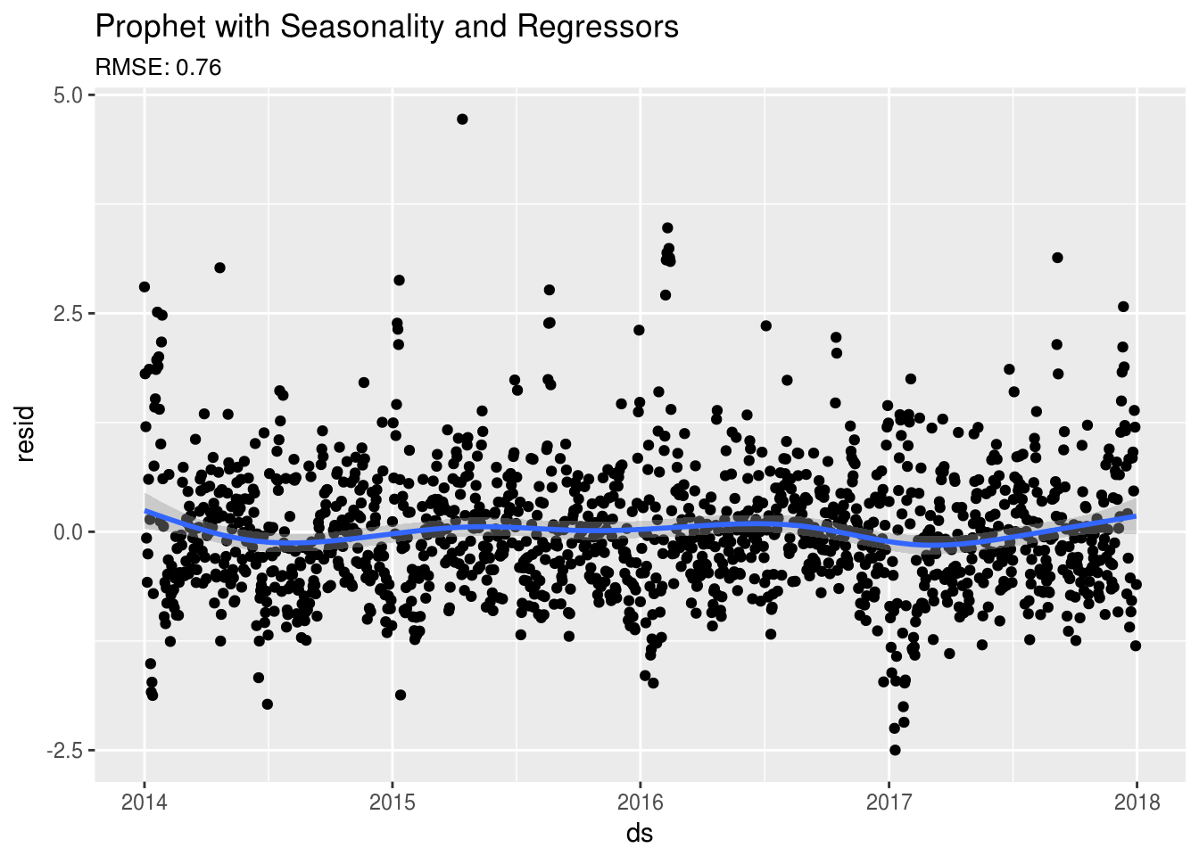

Cross-Validation Comparison of Models

Okay, now that we’ve gone over the basics of each of the models as well as assessing the model fit, let’s compare how well the models predict future PM2.5 levels. This cross validation is performed by assigning a rolling window in our time series. We split this window into two pieces, the “initial” time period and the “horizon”. We fit our model using the initial time period and compare our prediction of the horizon to its actual values. I picked the RMSE as my loss function in evaluating predictive performance.

A typical comparison is to compute the RMSE for each of the days in your horizon by combining all the differences between ‘y’ and ‘yhat’ from each of your rolling validations:

# RMSE by horizon
all.cv %>% 
  group_by(model,day) %>% 
  summarise(rmse=sqrt(mean((y-yhat)^2))) %>% 
  ggplot(.,aes(x=day,y=rmse,group=model,color=model)) +
  geom_line(alpha=.75) + geom_point(alpha=.75)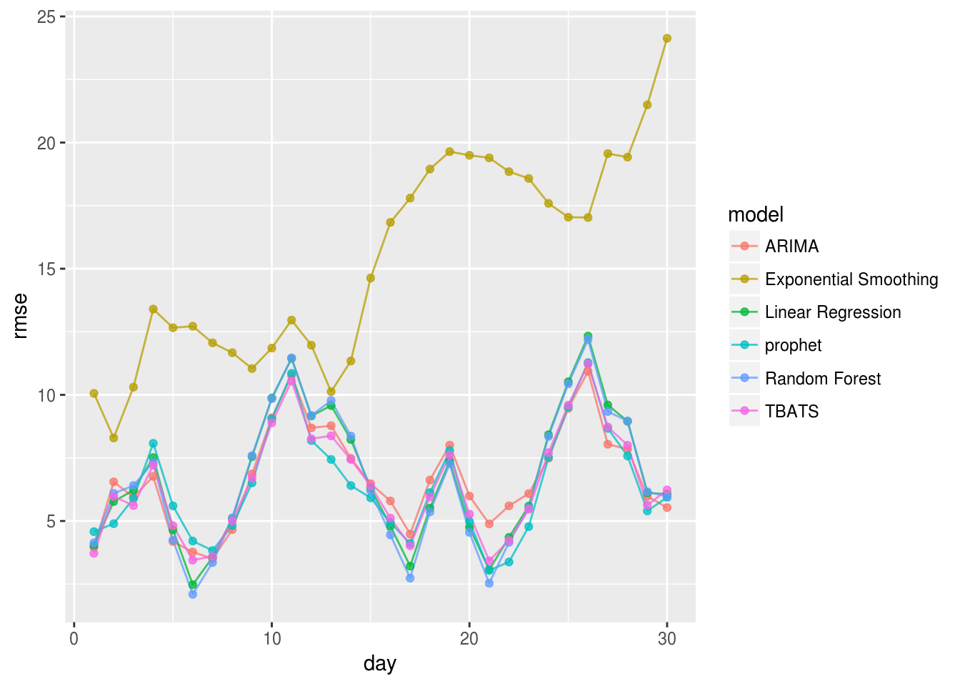

This is definitely an interesting result. Clearly the Exponential Smoothing model is not the best predictor with this data. Also, when comparing how well each model predicts future events, it appears that the OLS and Random Forest regression models perform just as well as the TBATS, ARIMA, and prophet models. In the plot below, we can also take a look at how each of these forecasted data looks like for the year of 2017.

# Prediction behaviors of different methods
ggplot(all.cv,aes(date,yhat,group=as.factor(cutoff),color=as.factor(cutoff)))+
  geom_line()+
  geom_line(aes(y=y),color="black",alpha=.15)+#geom_point(aes(y=y),color="black",alpha=.15)+
  facet_wrap(~model)+ guides(color="none") +
  theme(axis.title.x=element_blank(),
        axis.text.x=element_blank(),
        axis.ticks.x=element_blank())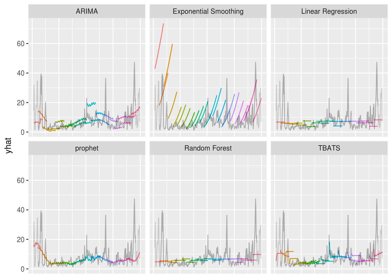

Some of the things that you’ll probably notice first off is:

• The reason the Exponental Smoothing model didn’t perform so well.
• Since I don’t know the future regressors’ values for OLS and Random Forest regression, I just set them to the values at the end of each initial window, which resulted in straight line forecasts.
• ARIMA appears to not be as robust as other methods.

Conclusion

Of all these methods, I would probably decide on either the TBATS or prophet model in forecasting future data. I hope you have enjoyed these exercises and intro to time series in R!

Where to learn more?

• FutureLearn Forecasting MOOC
• Forecasting: Principles and Practice
• Prophet: Forecasting at Scale

References

Hyndman, R.J. and Athanasopoulos, G. (2013) Forecasting: principles and practice. OTexts: Melbourne, Australia. http://otexts.org/fpp/. Accessed on February 11, 2018.

National Center for Environmental Information. Climate Data Online available at https://www.ncdc.noaa.gov/cdo-web. Accessed February 11, 2018.

Sean Taylor and Ben Letham (2017). prophet: Automatic Forecasting Procedure. R package version 0.2.1.9000. https://facebook.github.io/prophet/.

US Environmental Protection Agency. Air Quality System Data Mart [internet database] available at http://www.epa.gov/ttn/airs/aqsdatamart. Accessed?February 11, 2018.