Recently at work I’ve been asked to help some clinicians understand why my risk model classifies specific patients as high risk. Just prior to this work I stumbled across the work of some data scientists at the University of Washington called lime. LIME stands for “Local Interpretable Model-Agnostic Explanations”. The idea is that I can answer those questions I’m getting from clinicians for a specific patient by locally fitting a linear (aka “interpretable”) model in the parameter space just around my data point. I decided to pursue lime as a solution and the last few months I’ve been focusing on implementing this explainer for my risk model. Happily, I also discovered an R package that implements this solution that originated in python.
Sample Data
So the first step to this blog was to find some public data for illustration. I remembered an example used in an Introduction to Statistical Learning by James, Witten, Hastie and Tibshirani. I will use the Heart.csv data which can be downloaded using the link in the code below:
library(readr)
library(ranger)
library(tidyverse)
library(lime)

dat <- read_csv("http://www-bcf.usc.edu/~gareth/ISL/Heart.csv")
dat$X1 <- NULL
Now let’s take a quick look at the data:
Hmisc::describe(dat)## dat
##
## 14 Variables 303 Observations
## ---------------------------------------------------------------------------
## Age
## n missing distinct Info Mean Gmd .05 .10
## 303 0 41 0.999 54.44 10.3 40 42
## .25 .50 .75 .90 .95
## 48 56 61 66 68
##
## lowest : 29 34 35 37 38, highest: 70 71 74 76 77
## ---------------------------------------------------------------------------
## Sex
## n missing distinct Info Sum Mean Gmd
## 303 0 2 0.653 206 0.6799 0.4367
##
## ---------------------------------------------------------------------------
## ChestPain
## n missing distinct
## 303 0 4
##
## Value asymptomatic nonanginal nontypical typical
## Frequency 144 86 50 23
## Proportion 0.475 0.284 0.165 0.076
## ---------------------------------------------------------------------------
## RestBP
## n missing distinct Info Mean Gmd .05 .10
## 303 0 50 0.995 131.7 19.41 108 110
## .25 .50 .75 .90 .95
## 120 130 140 152 160
##
## lowest : 94 100 101 102 104, highest: 174 178 180 192 200
## ---------------------------------------------------------------------------
## Chol
## n missing distinct Info Mean Gmd .05 .10
## 303 0 152 1 246.7 55.91 175.1 188.8
## .25 .50 .75 .90 .95
## 211.0 241.0 275.0 308.8 326.9
##
## lowest : 126 131 141 149 157, highest: 394 407 409 417 564
## ---------------------------------------------------------------------------
## Fbs
## n missing distinct Info Sum Mean Gmd
## 303 0 2 0.379 45 0.1485 0.2538
##
## ---------------------------------------------------------------------------
## RestECG
## n missing distinct Info Mean Gmd
## 303 0 3 0.76 0.9901 1.003
##
## Value 0 1 2
## Frequency 151 4 148
## Proportion 0.498 0.013 0.488
## ---------------------------------------------------------------------------
## MaxHR
## n missing distinct Info Mean Gmd .05 .10
## 303 0 91 1 149.6 25.73 108.1 116.0
## .25 .50 .75 .90 .95
## 133.5 153.0 166.0 176.6 181.9
##
## lowest : 71 88 90 95 96, highest: 190 192 194 195 202
## ---------------------------------------------------------------------------
## ExAng
## n missing distinct Info Sum Mean Gmd
## 303 0 2 0.66 99 0.3267 0.4414
##
## ---------------------------------------------------------------------------
## Oldpeak
## n missing distinct Info Mean Gmd .05 .10
## 303 0 40 0.964 1.04 1.225 0.0 0.0
## .25 .50 .75 .90 .95
## 0.0 0.8 1.6 2.8 3.4
##
## lowest : 0.0 0.1 0.2 0.3 0.4, highest: 4.0 4.2 4.4 5.6 6.2
## ---------------------------------------------------------------------------
## Slope
## n missing distinct Info Mean Gmd
## 303 0 3 0.798 1.601 0.6291
##
## Value 1 2 3
## Frequency 142 140 21
## Proportion 0.469 0.462 0.069
## ---------------------------------------------------------------------------
## Ca
## n missing distinct Info Mean Gmd
## 299 4 4 0.783 0.6722 0.9249
##
## Value 0 1 2 3
## Frequency 176 65 38 20
## Proportion 0.589 0.217 0.127 0.067
## ---------------------------------------------------------------------------
## Thal
## n missing distinct
## 301 2 3
##
## Value fixed normal reversable
## Frequency 18 166 117
## Proportion 0.060 0.551 0.389
## ---------------------------------------------------------------------------
## AHD
## n missing distinct
## 303 0 2
##
## Value No Yes
## Frequency 164 139
## Proportion 0.541 0.459
## ---------------------------------------------------------------------------Our target variable in this data is AHD. This flag identifies whether or not a patient has Coronary Artery Disease. If we can predict this accurately, clinicians could probably better treat these patients and hopefully help them avoid the symptoms of AHD like chest pain or worse, heart attacks.
Data Wrangling
For a predictive model I’ve opted to use a random forest model using the ranger implmentation which parallelizes the random forests algorithm in R. But first, some data cleaning is necessary. After replacing missing values, I’m going to split the data into test and training dataframes.
# Replace missing values
dat$Ca[is.na(dat$Ca)] <- -1
dat$Thal[is.na(dat$Thal)] <- "missing"

## 75% of the sample size
smp_size <- floor(0.75 * nrow(dat))

## set the seed to make your partition reproducible
set.seed(123)
train_ind <- sample(seq_len(nrow(dat)), size = smp_size)

train <- dat[train_ind, ]
test <- dat[-train_ind, ]

mod <- ranger(AHD~., data=train, probability = TRUE, importance = "permutation")

mod$prediction.error
## [1] 0.1326235Our quick and dirty check of the OOB prediction error tells us that our model appears to be doing okay at predicting AHR. Now the trick is to describe to our physicians and nurses why we believe someone is high risk for AHR. Before I learned of lime, I would have probably done something similar to the code below by first looking at which variables were most important in my trees.
plot_importance <- function(mod){
  tmp <- mod$variable.importance
  dat <- data.frame(variable=names(tmp),importance=tmp)
  ggplot(dat, aes(x=reorder(variable,importance), y=importance))+
    geom_bar(stat="identity", position="dodge")+ coord_flip()+
    ylab("Variable Importance")+
    xlab("")
}

# Plot the variable importance
plot_importance(mod)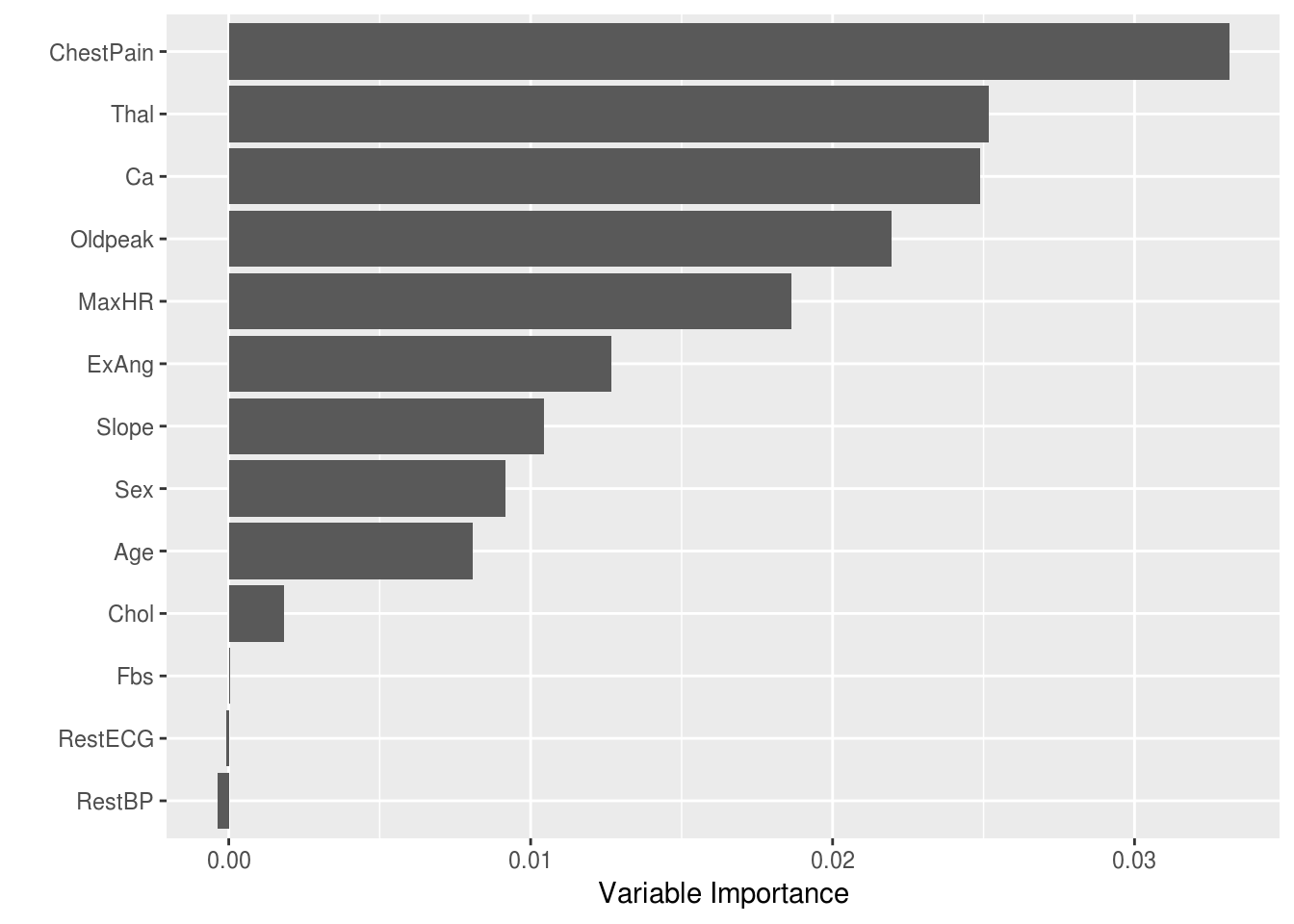
After this, I probably would have taken a look at some partial dependence plots to get an idea of how those important variables are changing over the range of that variable. However, often the weakness of this approach is that I need to hold all other variables constant. And if I truly believe there are interactions between my variables, the partial dependence plot could change dramatically when other variables are changed.
Explain the model with LIME
Enter lime. As discussed above, the entire purpose of lime is to provide a local interpretable model to help us understand how our prediction would change if we tweak the other variables slightly in a lot of permutations. The first step to using lime in this specific case is to add some functions so that the lime package knows how to deal with the output of the ranger package. Once I have these I can use the combination of the lime() and explain() functions to get what I need. As in all multivariate linear models, we still have an issue… correlated explanatory varaibles. And depending on the number of variables in our original model, we may need to pair down our models to only look at the most “influential” or “important” variables. By default lime is going to use either forward-selection or pick the variables with the larges coefficients after correcting for multicollinearity using ridge regression or L2 penalization. As seen below, you can also select variables for the explanation using Lasso (aka L1 penalization) or use xgboost most important variables using the "tree" method.
# Train LIME Explainer
expln <- lime(train, model = mod)


preds <- predict(mod,train,type = "response")
# Add ranger to LIME
predict_model.ranger <- function(x, newdata, type, ...) {
  res <- predict(x, data = newdata, ...)
  switch(
    type,
    raw = data.frame(Response = ifelse(res$predictions[,"Yes"] >= 0.5,"Yes","No"), stringsAsFactors = FALSE),
    prob = as.data.frame(res$predictions[,"Yes"], check.names = FALSE)
  )
}

model_type.ranger <- function(x, ...) 'classification'


reasons.forward <- explain(x=test[,names(test)!="AHD"], explainer=expln, n_labels = 1, n_features = 4)
reasons.ridge <- explain(x=test[,names(test)!="AHD"], explainer=expln, n_labels = 1, n_features = 4, feature_select = "highest_weights")
reasons.lasso <- explain(x=test[,names(test)!="AHD"], explainer=expln, n_labels = 1, n_features = 4, feature_select = "lasso_path")
reasons.tree <- explain(x=test[,names(test)!="AHD"], explainer=expln, n_labels = 1, n_features = 4, feature_select = "tree")
Note: Using the current version of lime you may have issues with the feature_select = "lasso_path" option. To get the above code to run above you can install my tweaked version of lime here.
Plotting explanations
Now that we have all the explanations, one of my favorite features in the lime package is the plot_explanations() function. You can easily show the most important variables for each of our selection methods above and we can see that they are all very consistent in the choice of the top 4 most influential variables in predicting AHD.
plot_explanations(reasons.forward)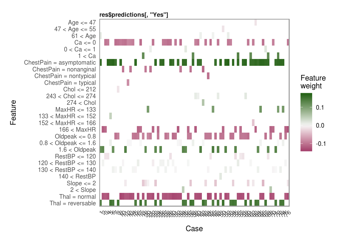
plot_explanations(reasons.ridge)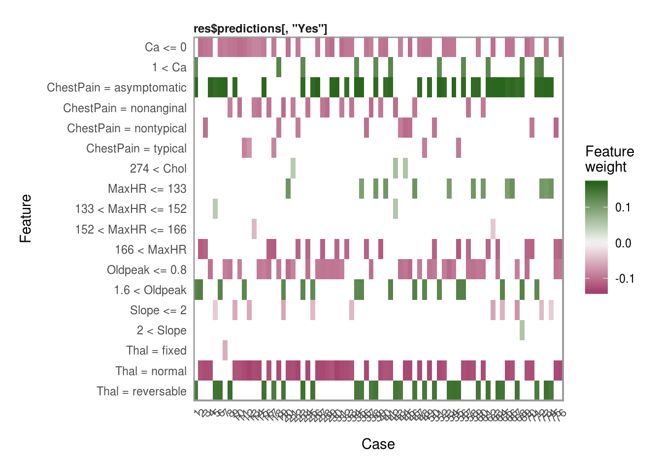
plot_explanations(reasons.lasso)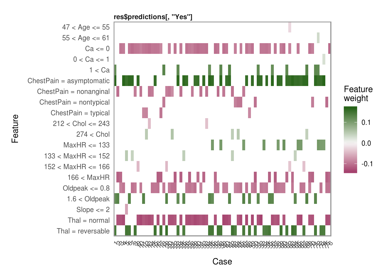
plot_explanations(reasons.tree)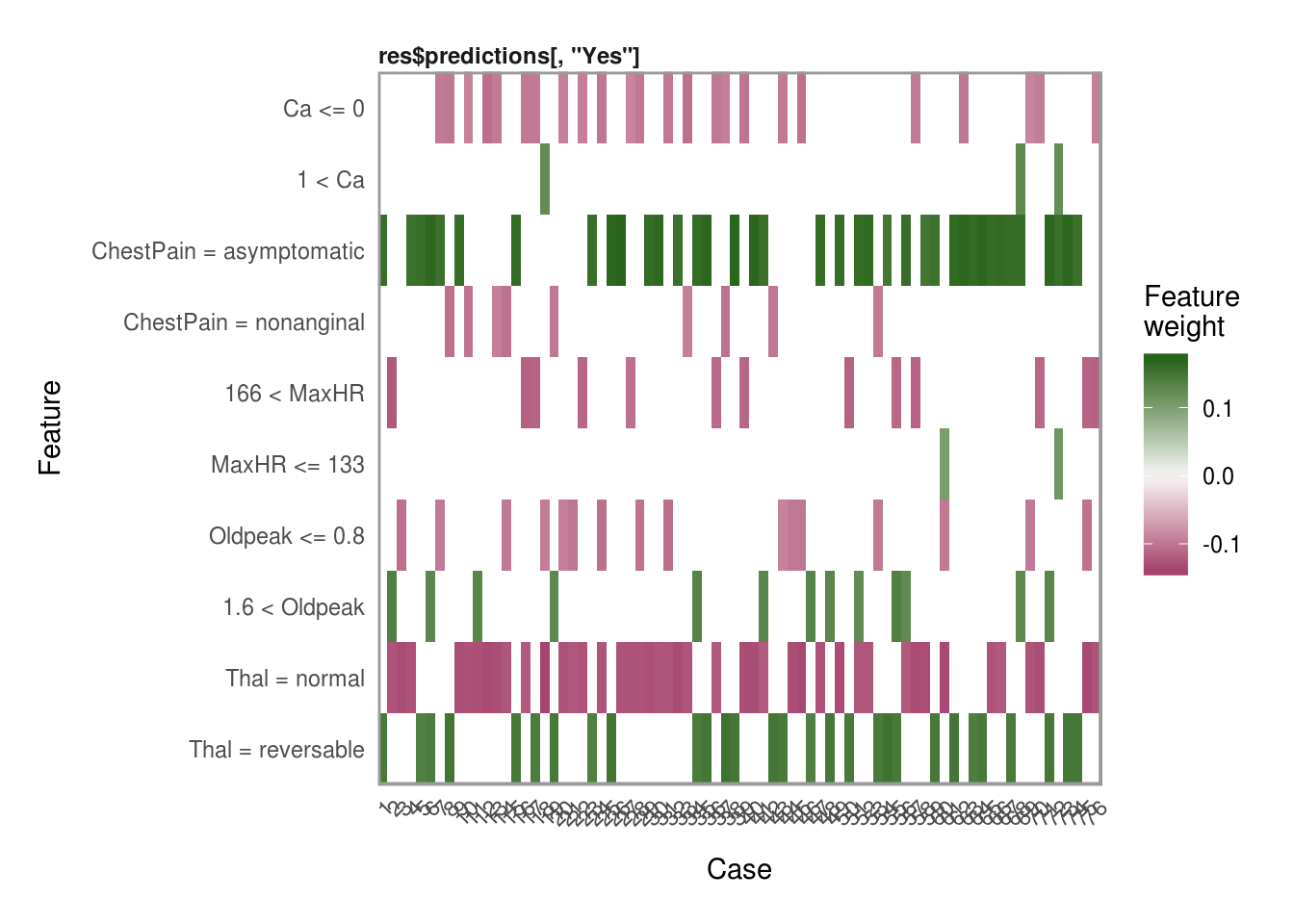
Thanks for reading this quick tutorial on lime. There is much more of this package that I want to explore. Particulary its use for image and text classifications. Then the only real question left is… How do I get one of those cool hex stickers for lime? ;)
